
The sheer amount of data available on the Internet has already grown beyond imagination and is continuing to grow exponentially through the rise of Social Media and Artificial Intelligence. This trend puts techniques for duplicate detection and deduplication on the agenda for many companies, and especially so in the Media Monitoring business.
To keep track of news and conversations around the globe, we crawl millions of online news, social media posts and broadcasts every day. By applying duplicate detection algorithms to all of that data we keep NewsRadar® lean and fast, making it easy for users to understand what the conversation is all about in real-time. Let’s have a look behind the curtain of content deduplication at pressrelations.
The case for deduplicating millions of documents in real-time
There’s a wide variety of use cases for duplicate detection in the field of Media Monitoring, ranging from Virality Analyses and Content Distribution Tracking to Plagiarism Detection and Web Crawling. Some of these tasks require content to be tracked in a byte-wise manner and are easily handled with conventional hash algorithms like MD5 or SHA, but other use cases require deduplicating content with a degree of fuzziness, focussing on the story and it’s context while ignoring the exact spelling and phrasing. What we’re looking for in these scenarios aren’t exact duplicates, but near-duplicates.
Conventional near-duplicate detection
There are many ways to detect near-duplicate content, the most popular one being K-means clustering. K-means represents all documents to be analyzed as high-dimensional vectors and measures the Euclidean distance between those vectors. It then assigns the documents into k clusters while trying to minimize the distance of each document to the clusters center document.
Unfortunately this approach has linear complexity and is prohibitively slow when applied to big data sets ranging in the millions of documents and is therefore not appropriate for real-time use cases. Furthermore it requires users to choose the desired number of clusters up front and forces documents to fit into those clusters no matter the actual degree of similarity. Instead we employ a fingerprint based algorithm called MinHash.
The magic of MinHash
MinHash works quite differently since it treats documents as a set of shingles, specifically the set of all k-shingles from a document. Let’s look at a simple document with varying values of k to understand what that means:
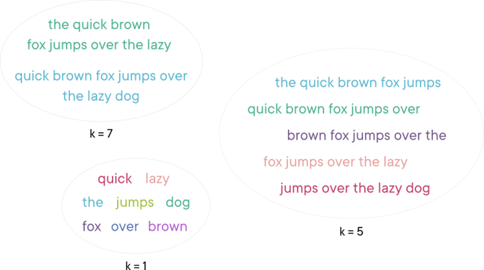
Treating documents as sets of shingles allows measuring their similarity by computing the Jaccard similarity, which is the amount of shared shingles between two documents relative to the document size. A high number of shared shingles means that the documents are likely to be similar to each other as long as k is chosen appropriately. Small values lead to more false positives by being unspecific, while large values lead to more false negatives since it’s less likely for long phrases to reappear in other documents. Internal tests have shown that k = 5 yields good results for average text sizes of 4 kB, but your mileage may vary based on the features of your data. Take your time tuning this value with regards to your data since it has a large impact on how fuzzy the matching will be.
Computing the Jaccard similarity between millions of documents in real-time wouldn’t be possible though, and this is where the magic of the MinHash algorithm comes into play. Let’s assume that documents d1 and d2 have a Jaccard similarity of 0.8 (80%), and h(d) is a hash function over all shingles from a document D, then the probability of h(d1) = h(d2) is also 0.8 (see “Mining of Massive Datasets”, chapter 3.3.3 for a detailed explanation). If p(h(d1) = h(d2)) = 0.8, then the documents share 80% of their shingles, but our algorithm needs to reach a binary decision for it to be useful – are the documents actually similar enough or not?
A single hash function can only answer this question in probabilistic terms, but a set of different hash functions, each fulfilling p(h(d1) = h(d2)) = 0.8, will indeed yield 80% functions that equal values. Given that property, we can identify near-duplicates by looking for a certain amount of matching hash values. You could choose just about any set of hash functions for MinHash, but it’s best to go for a lightweight algorithm like Murmur3 which is CPU efficient and can be seeded to generate dozens of unique hash functions. Assuming you choose to go for 200 hash functions, the result would look like this:
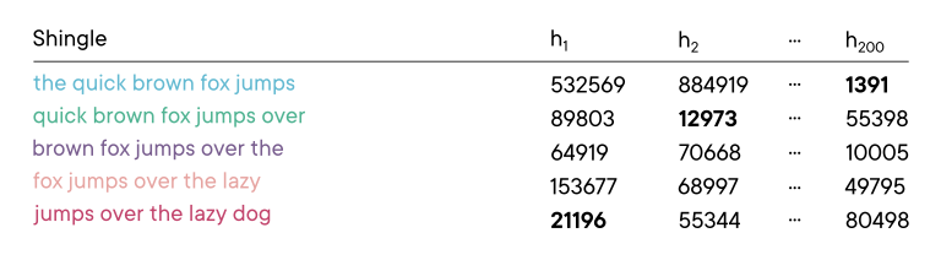
Notice how each column of hash functions has a bold value? Each hash function hashes each shingle independently and only the minimum value per hash function is kept in the end, effectively making for a pseudo-random shingle selection. This it what puts the Min into MinHash and makes up the final fingerprint. In our example, that would we 21196 12973 … 1391. In other words, the document is represented by the shingles “jumps over the lazy dog”, “quick brown fox jumps over” and “the quick brown fox jumps” (omitting the shingles picked by h3 to h199 of course).
Finding similar documents in the blink of an eye
Finding similar documents requires finding documents with a similar fingerprint, that is with similar shingles. If we were to require a 75% match between fingerprints in a SQL based system working with 200 hash functions, the query would need to look for all possible subsets of cardinality 150, totaling 10⁴⁷ combinations of hashes to match:
SELECT doc_id
FROM fingerprints
WHERE
(hash_1 = h1 AND hash_2 = h2 … AND hash_150 = h150) OR
(hash_1 = h1 AND hash_3 = h3 … AND hash_151 = h151) OR
(hash_1 = h1 AND hash_4 = h4 … AND hash_152 = h152) OR
…
This isn’t really what you’d expect to be lightning fast, right? Clearly we need another way to handle the queries in our database, and Locality Sensitive Hashing (LSH) is one way to achieve this with a probabilistic approach. It groups hashes into bands and hashes those bands, so instead of 200 hashes, you end up with just 20 bands consisting of 10 hashes each. A simple example with 6 hash functions and 2 bands would look like this:
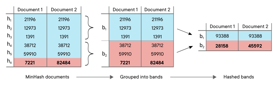
Naturally this leads to data compresses since it reduces the number of bytes required to store a fingerprint. But much more importantly, it combines loosely related pieces of information into bigger chunks, thereby establishing relationships between hash values, allowing us to find documents with lot’s of matching hashes in one fell swoop. After this process it’s possible to identify near-duplicates candidates by looking for just a single band match between documents – we no longer need to check 10⁴⁷ combinations of hashes, but just 20 bands:
SELECT doc_id
FROM fingerprints
WHERE band_1 = b1 OR band_2 = b2 … OR band_n = bn
Did you notice that we’ve been talking about near-duplicates all the time and now it’s suddenly near-duplicate candidates? There had to be a trick somewhere, and this is exactly it. LSH cannot reliably answer the question of whether or not two documents are near-duplicates, but it can be fine-tuned to keep the rate of false negatives/positives within very reasonable limits. The number of hashes and bands directly affects the likelihood of detecting actual near-duplicate candidates after applying LSH:
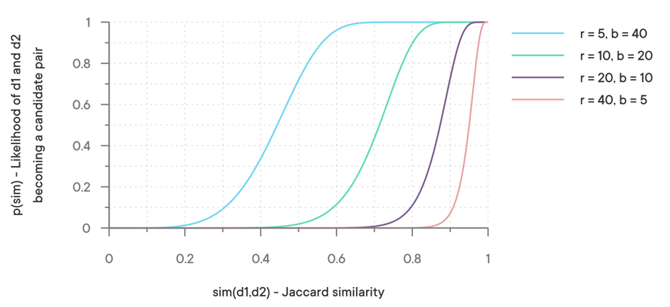
If you take a look at the third S-curve from the left (r = 20 and b = 10), you’ll see that only documents with Jaccard similarity >= 0.7 have a chance to become near-duplicate candidates, but it’s still very low at 0.795%. At a Jaccard similarity of 0.9 the likelihood to detect near-duplicate candidates is already 73%, and at 0.95 it climbs up to 99%. After some testing we decided to use exactly those parameters, but depending on the use case you might very well choose to use a different set of parameters using this function:
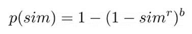
Just remember that LSH computes near-duplicate candidates so you might want to check those candidates for actual Jaccard similarity in a pairwise manner before declaring them as similar (in memory, after querying the candidates from the database).
Making it fly in production
Let’s talk a bit about the tech that makes MinHash and LSH fly at pressrelations before wrapping it up. After several iterations with Ruby, Python and SQL, we finally landed at a solution that incorporates Elixir, Rust, Elasticsearch and SQL Server for easy scalability and top notch performance:
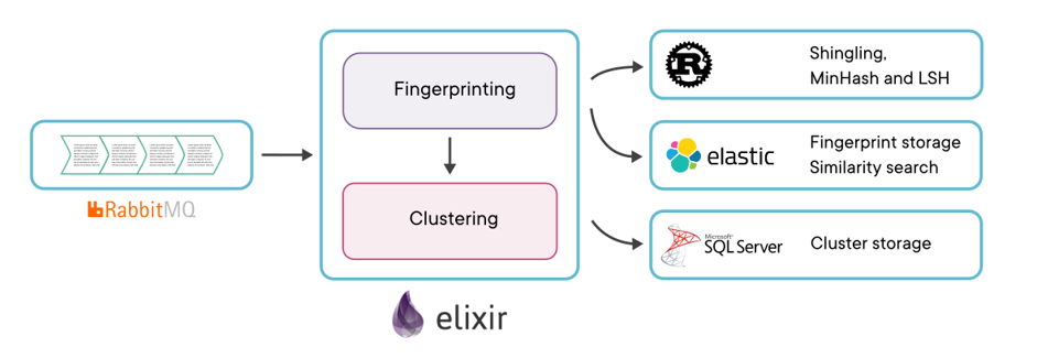
Elixir powers our microservice handling documents to be deduplicated from a RabbitMQ queue, hands off the hard computing work to Rust and sends fingerprints to Elasticsearch for fast storage and retrieval. Upon receiving new documents, it finds all the similar documents from Elasticsearch via band matches, retrieves their cluster IDs from the database and chooses the best existing cluster for the new document (based upon cluster size and age). It then updates the cluster by simply copying the chosen cluster ID to the new document.
Calculating hundreds of billions of hashes per day meant that we needed to find the fastest implementation of Murmur3, and that’s how we landed at Rust and it’s fantastic crate fasthash. It’s already optimized for the prevalent CPU architectures and is able to compute millions of hashes per second. And the integration of Rust and Elixir is a blaze with Elixir’s rustler hex, making for easy maintenance of the solution in the long term.
Wrapping it up
We’ve covered a lot of ground in this blog post, starting off by motivating the need for algorithms like MinHash / LSH, explaining their inner workings and demonstrating the feasibility of real-time deduplication with streams in the order of millions of items. Of course we couldn’t do all of this by ourselves, so here’s a list of sources that we found invaluable while working on this topic. Stay tuned for more “behind the scenes” posts straight from our tech team.
List of sources
- Anand Rajaraman,
Jure Leskovec, and Jeffrey D. Ullman. Mining
of Massive Datasets (PDF) - https://towardsdatascience.com/understanding-locality-sensitive-hashing-49f6d1f6134
- https://moz.com/devblog/near-duplicate-detection
- https://en.wikipedia.org/wiki/Jaccard_index
Photo by chuttersnap on Unsplash